This guide walks through how vector databases enable similarity search, from the fundamental concept of embeddings to the indexing strategies that power large-scale retrieval systems.
You'll learn:
How embeddings transform unstructured data into searchable vectors
How vector databases handle nearest neighbor search, metadata filtering, and hybrid retrieval
How indexing techniques like HNSW, IVF, and PQ make vector search scalable in production
Vector Databases Explained in 3 Levels of Difficulty
Image by Author
Introduction
Traditional databases answer exact questions: does a record matching these criteria exist? Vector databases answer a fundamentally different one: which records are most similar to this? That distinction matters because most modern data—documents, images, user behavior, audio—can't be searched by exact match. The right query isn't "find this," but "find what resembles this." Embedding models enable this by converting raw content into vectors where geometric proximity maps to semantic similarity.
The challenge is scale. Comparing a query vector against every stored vector means billions of floating-point operations at production data volumes, making real-time search impractical. Vector databases address this with approximate nearest neighbor algorithms that skip most candidates while still returning results nearly identical to exhaustive search, at a fraction of the computational cost.
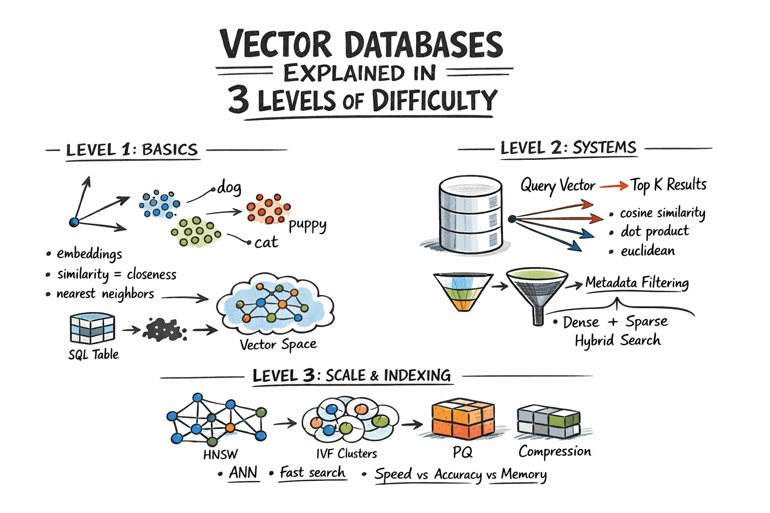
This article breaks down how that works across three levels: the core similarity problem and what vectors enable, how production systems store and query embeddings with filtering and hybrid search, and the indexing algorithms and architectural decisions that make it work at scale.
Level 1: Understanding the Similarity Problem
Traditional databases store structured data—rows, columns, integers, strings—and retrieve it with exact lookups or range queries. SQL handles this efficiently. But much real-world data isn't structured. Text documents, images, audio, and user behavior logs don't fit neatly into columns, and "exact match" is the wrong query model for them.
The solution is representing this data as vectors: fixed-length arrays of floating-point numbers. An embedding model like OpenAI's text-embedding-3-small, or a vision model for images, converts raw content into a vector capturing its semantic meaning. Similar content produces similar vectors. The word "dog" and "puppy" end up geometrically close in vector space. A photo of a cat and a drawing of a cat also cluster together.
A vector database stores these embeddings and enables similarity search: "find the 10 vectors closest to this query vector." This is nearest neighbor search.
Level 2: Storing and Querying Vectors
Embeddings
Before a vector database can operate, content must be converted into vectors. This happens through embedding models—neural networks that map input into dense vector space, typically with 256 to 4096 dimensions depending on the model. The specific numbers in the vector lack direct interpretation; what matters is the geometry: close vectors indicate similar content.
You call an embedding API or run a model locally, receive an array of floats, and store that array alongside your document metadata.
Distance Metrics
Similarity is measured as geometric distance between vectors. Three metrics dominate:
Cosine similarity measures the angle between vectors, ignoring magnitude. Common for text embeddings where direction matters more than length.
Euclidean distance measures straight-line distance in vector space. Useful when magnitude carries semantic weight.
Dot product is computationally fast and works well with normalized vectors. Many embedding models are trained specifically for it.
The metric choice should align with how your embedding model was trained. Mismatched metrics degrade result quality.
The Nearest Neighbor Problem
Finding exact nearest neighbors is straightforward in small datasets: compute distance from the query to every vector, sort results, and return the top K. This is brute-force or flat search, and it's 100% accurate. It also scales linearly with dataset size. At 10 million vectors with 1536 dimensions each, flat search becomes too slow for real-time queries.
The solution is approximate nearest neighbor (ANN) algorithms. These trade minimal accuracy for substantial speed gains. Production vector databases run ANN algorithms under the hood. The specific algorithms, their parameters, and their tradeoffs are examined in the next level.
Metadata Filtering
Pure vector search returns the most semantically similar items globally. In practice, you typically need: "find the most similar documents belonging to this user created after this date." That's hybrid retrieval: vector similarity combined with attribute filters.
Implementations vary. Pre-filtering applies the attribute filter first, then runs ANN on the remaining subset. Post-filtering runs ANN first, then filters results. Pre-filtering is more accurate but more expensive for selective queries. Most production databases use variants of pre-filtering with intelligent indexing to maintain speed.
Hybrid Search: Dense + Sparse
Pure dense vector search can miss keyword-level precision. A query for "GPT-5 release date" might semantically drift toward general AI topics rather than the specific document containing the exact phrase. Hybrid search combines dense ANN with sparse retrieval (BM25 or TF-IDF) to capture both semantic understanding and keyword precision.
The standard approach runs dense and sparse search in parallel, then merges scores using reciprocal rank fusion (RRF)—a rank-based merging algorithm that doesn't require score normalization. Most production systems now support hybrid search natively.
Level 3: Indexing for Scale
Approximate Nearest Neighbor Algorithms
Three leading approximate nearest neighbor algorithms represent distinct points along the speed-memory-recall tradeoff curve, each optimized for different use cases.
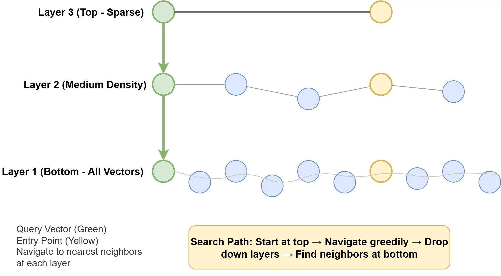
Hierarchical navigable small world (HNSW) constructs a multi-layered graph structure in which vectors serve as nodes connected by edges to similar neighbors. Sparse upper layers enable rapid long-distance navigation, while denser lower layers provide fine-grained local search precision. Query execution involves traversing this graph structure toward the closest matches. HNSW offers exceptional speed and recall but demands substantial memory, making it the default choice in many contemporary vector databases.
How Hierarchical Navigable Small World Works
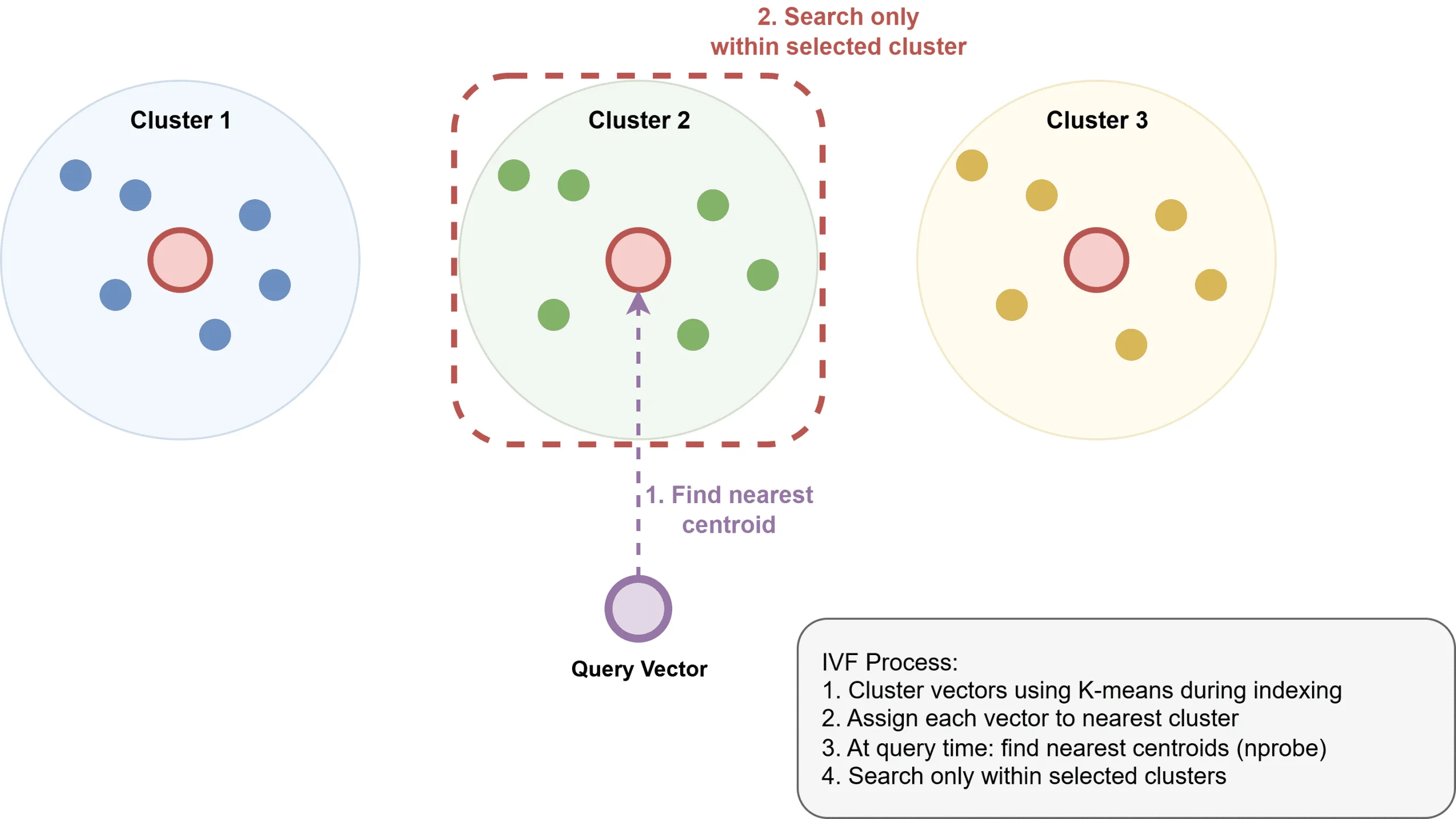
Inverted file index (IVF) partitions vectors into clusters via k-means clustering, creates an inverted index mapping clusters to their constituent vectors, and limits search operations to the most relevant clusters. While IVF consumes less memory than HNSW, it typically exhibits slower query performance and necessitates an upfront training phase for cluster generation.
How Inverted File Index Works
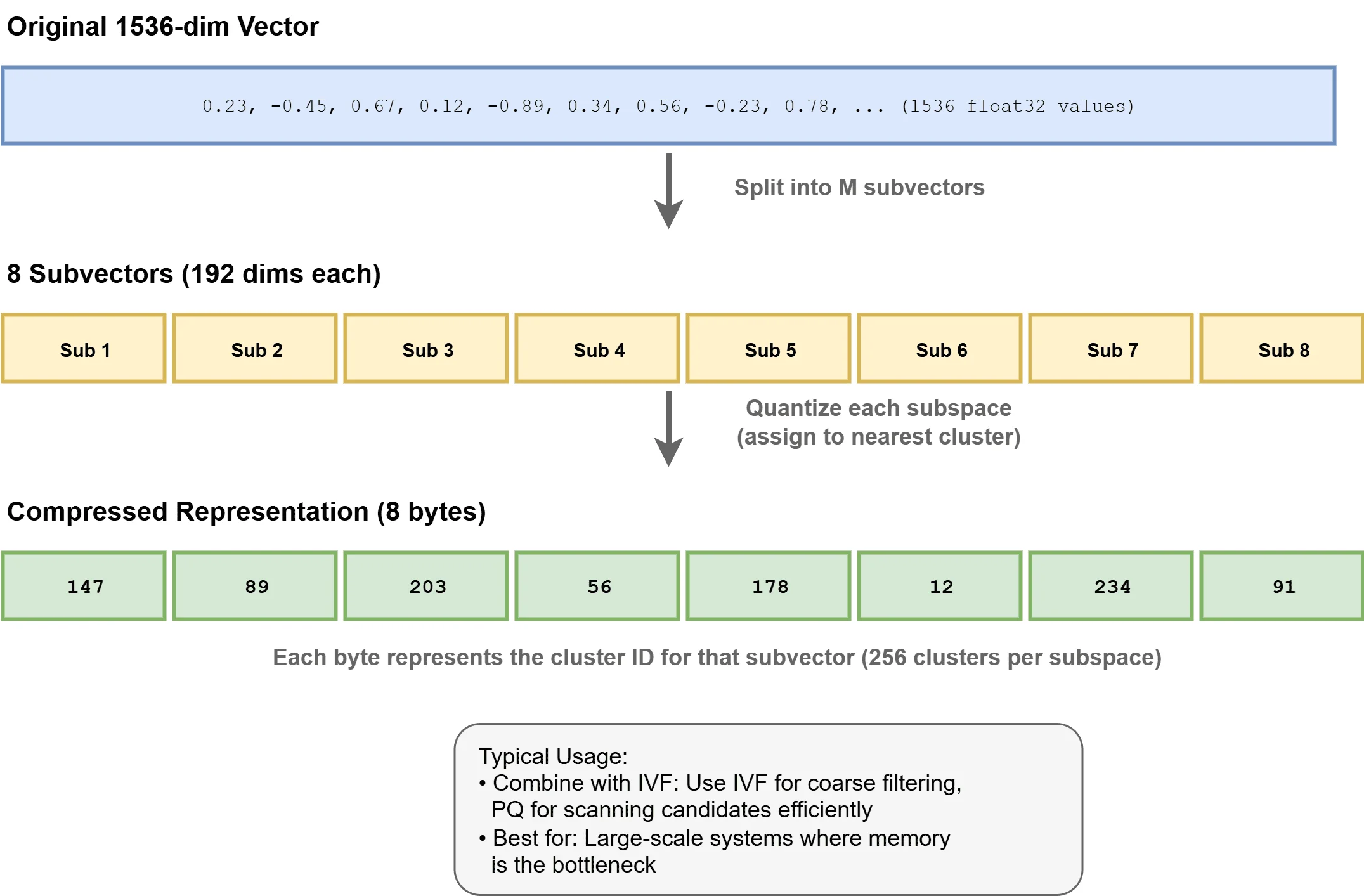
Product Quantization (PQ) achieves compression by segmenting vectors into subvectors and quantizing each against a learned codebook. This technique can slash memory requirements by 4–32x, making billion-scale deployments feasible. PQ frequently pairs with IVF in hybrid IVF-PQ configurations, as implemented in systems like Faiss.
How Product Quantization Works
Index Configuration
HNSW exposes two primary configuration parameters: ef_construction and M:
ef_construction determines the candidate pool size during index building. Larger values typically enhance recall but extend construction time.
M specifies the number of bidirectional connections per node. Increasing M often boosts recall while consuming additional memory.
These parameters should be calibrated according to your specific recall targets, latency requirements, and available memory.
The query-time parameter ef_search governs candidate exploration breadth. Raising this value improves recall at the expense of query latency, and it can be adjusted dynamically without index reconstruction.
ANN algorithms operate along a fundamental tradeoff curve. Higher recall invariably requires searching more index regions, which translates directly to increased latency and computational cost. Benchmark performance against your actual data distribution and query workload. A recall@10 of 0.95 may suffice for search applications, while recommendation engines might demand 0.99 or higher.
Scale and Sharding
A single in-memory HNSW index typically accommodates 50–100 million vectors on one machine, depending on vector dimensionality and available RAM. Beyond this threshold, sharding becomes necessary: the vector space is partitioned across multiple nodes, queries are distributed to relevant shards, and results are aggregated. This approach introduces coordination complexity and requires thoughtful shard key design to prevent load imbalances. For deeper exploration, consult How does vector search scale with data size?
Storage Backends
Vector indexes commonly reside in RAM to maximize ANN search performance. Associated metadata typically lives in separate key-value or columnar stores. Some implementations leverage memory-mapped files to handle datasets exceeding available RAM, paging to disk as needed—a strategy that trades latency for capacity.
Disk-native ANN indexes like DiskANN (from Microsoft Research) are engineered to operate directly from SSDs with minimal memory footprint. These systems deliver competitive recall and throughput for massive datasets where memory constraints are the primary bottleneck.
Vector Database Options
Vector search technologies cluster into three main categories.
First, purpose-built vector databases include:
Pinecone: a fully managed service requiring zero operational overhead
Qdrant: an open-source, Rust-based platform with advanced filtering capabilities
Weaviate: an open-source solution featuring integrated schema management and modular architecture
Milvus: a high-performance open-source database optimized for large-scale similarity search, offering distributed deployment and GPU acceleration
Second, traditional database extensions like pgvector for Postgres perform well at small to medium scale.
Annoy from Spotify, tuned for read-intensive workloads
For emerging retrieval-augmented generation (RAG) projects at moderate scale, pgvector represents a pragmatic starting point if Postgres is already in your stack, minimizing operational complexity. As requirements evolve—particularly with growing datasets or sophisticated filtering needs—Qdrant or Weaviate become increasingly attractive, while Pinecone suits teams prioritizing fully managed infrastructure.
Wrapping Up
Vector databases address a concrete challenge: locating semantically similar content at scale with low latency. The fundamental concept is elegant: represent content as vectors and search by distance. However, production deployment details—choosing between HNSW and IVF, tuning recall parameters, implementing hybrid search, and architecting sharding strategies—prove critical at scale.